Implementation of a simulator for different problems of molecular dynamics, including the Rayleigh-Taylor instability or the cooling process of Argon. I especially appreciated the affinity to physics, while having distinct aspects of software design/architecture, numerical methods and optimization opportunities. Created as part of my university practical course.

My personal contributions to this simulator focus primarily on the data structures used to contain particles, developer experience, sequential performance evaluation and optimization, some simulation reliability, as well as the implementation and evaluation of one full practical experiment.

Particle Containers

To store a large number of particles for processing, we utilized different types and container implementations, depending on the tradeoff between computational cost and physical accuracy. I additionally used this opportunity to apply different concepts from C++, to explore the language a bit.

Types

To store the position and velocity of particles, I first implemented the custom explicit type Vector for a mathematical vector instead of using std::array. I designed it as a templated class, which can be instantiated as a Vector of dimension N and elements of type T, to keep it flexible for different applications.

template <class T, size_t N>
    requires std::integral<T> || std::floating_point<T>
class Vector { ... };

It supports operations, implemented using operator overloading, such as

• access with subscript and structured bindings,
• point-wise arithmetic operations,
• inner product,
• euclidean norm,
• scalar multiplication, and
• comparison.

A Particle then groups properties such as its mass, type, current position, velocity and force acting on it, as well as other properties that are needed to nicely implement boundary conditions of the domain and different force types.

Concept VS Abstract Class

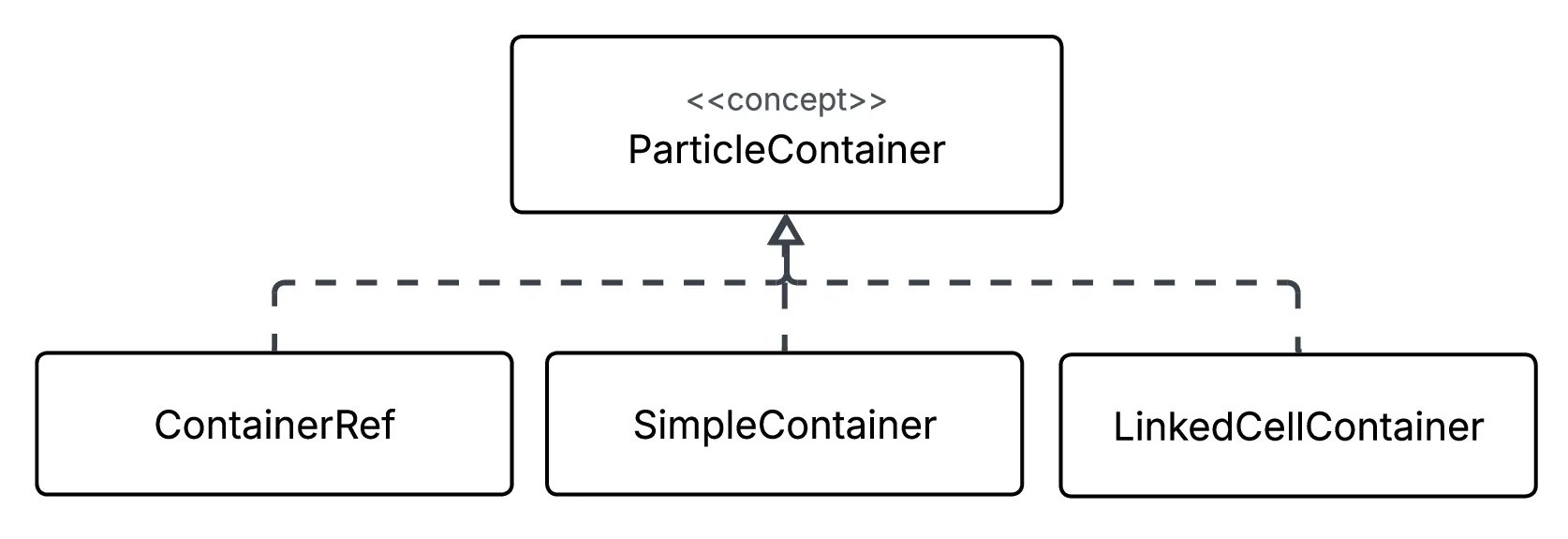
To store thousands of particles, I could have implemented an abstract class ParticleContainer

class ParticleContainer {...};

so that more specialized container implementations would inherit and override all methods. However, then all affected methods or classes would access the abstract type ParticleContainer at function call within the implementation, and the actual virtual function being called would be chosen at runtime via the vtable. As I wanted to keep my implementation flexible for certain simulations, but also not introduce unnecessary overhead at every container operation, I decided to look into C++ concepts

template <typename C>
concept ParticleContainer = requires(C c) {...};

The method requirements act similar to an interface, with specialized containers needing to implement them. For instance, any specialized container needed functions querying properties like the size of the container, or methods to access or add certain particles, or functions returning specialized iterators. The affected functions or classes then need to be implemented as a template, with a template parameter fulfilling the concept ParticleContainer. In their implementation, this template parameter acts like an abstract type, but is instantiated at compile time. As a result, the exact specialized function lookup happens at compile time, and not runtime of the simulation.

Containers

Concretely, I created multiple specialized containers, implementing the ParticleContainer requirements. They differ in how the particles are stored and managed internally.

Container Class SimpleContainer

This is the most naive implementation, with all particles being stored in a std::vector<Particle>. There is nothing special about it, so it is straightforward to implement. Despite being templated, it is absolutely not usable for larger simulations, as it misses optimizations for simplifying assumptions and as a result, for a force calculation (which is the most compute intensive part of a simulation) of a single Particle, will effectively iterate over all other Particles in the data structure.

Generic Type ContainerRef

This type was implemented to encapsulate a pointer to an arbitrary container implementing the concept ParticleContainer. It is used like a reference to a generic container, thus, essentially handrolling the indirection of a vtable. This data structure is NOT used for performance-critical segments, but rather functions—such as IO—we could not template.

Container Class LinkedCellContainer

This container utilizes the fact, that at a specific distance of two Particles, we can assume the forces between to be negligible. As a result, for the force calculation of a single Particle, it suffices to only consider other Particles within a certain radius. The LinkedCellContainer utilizes this assumption to not iterate over all Particles in the data structure and text whether they are in the radius—like the SimpleContainer needs to. Instead, it internally divides the domain into cells, and stores the Particles accordingly, so that only the neighboring cells of a Particle need to be iterated. This improves the runtime of the force calculation immensely, as it now takes linear instead of quadratic time, which we empirically verified.

As this container is more involved in its implementation, I want to present some thoughts I had while designing it.

I considered two approaches for the container architecture:

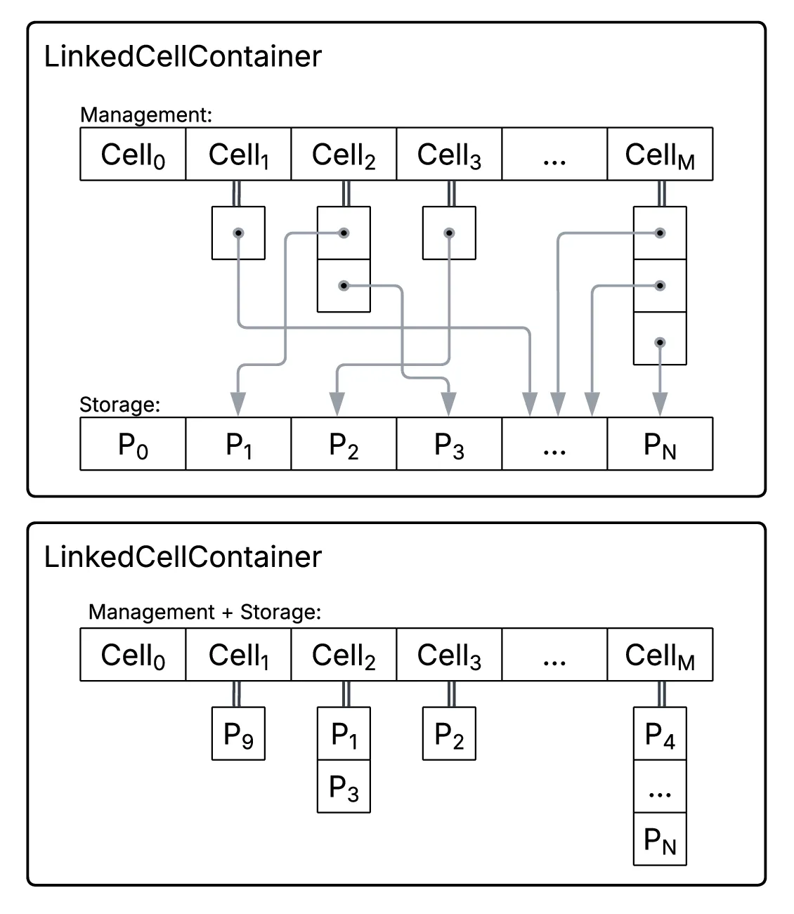
1.A) External Storage

Having an explicit std::vector for storing the Particles, and additional linearized std::vector for the cells, so that each cell only contains references to the Particles in the storage (see upper part of the picture above). As a result, when Particles change cells, one only needs to update the references in the cells, but iterating over the particles in concrete cells needs an indirect lookup via the storage.

1.B) Direct Storage

Within the linearized std::vector for the cells, each cell directly stores the Particles (see lower part of the picture above). As a result, moving particles from one cell to another entails moving all its data, however iterating over certain cells could directly access the relevant Particle properties.

I decided to go with approach A, as moving all Particle data in a very dynamic simulation seemed detrimental. So then I needed to decide in what form I wanted to reference the stored Particles. The references needed stay valid even after many container operations, they needed to enable a fast iteration to exploit memory locality of the storage, and they needed to enable a fast addition or removal of Particles. I then had the following options.

2.A) Pointers to Particles in the storage

Direct pointers to the elements in storage allow for a direct access of the Particle’s data. However, they also invalidate when the underlying storage std::vector resizes. A potential resize has to be caught at every addition or deletion of a Particle, and the revalidation takes linear time, which makes pointers problematic.

2.B) Indices of Particles in the storage

Indices to the elements do not invalidate when the std::vector resizes or when a Particle is added to the end of the storage. However, they require linear-time revalidation when a Particle is removed from the middle of the storage, and require an additional access though the storage data structure when accessing the Particle’s data.

2.C) Begin and End indices in the storage

Instead of addressing each Particle individually, one could also sort the Particles in the storage so that the elements belonging to a cell are laid-out as a block, to which the cell only stores its begin and end indices. Those two indices would not be invalidated at a storage resize, and the layout would allow for an efficient iteration over the Particles within a cell. However, it requires an ordered storage and a complex swapping of Particles at most addition or removals.

In the end, I decided to go with B due to complexity reasons, so that the last choice for me was to decide, which data structure I would use for the cells, that manage these indices. The data structure needed to maintain unique elements and stabile iterators over the indices, and also allow for an efficient iteration and removal or addition of an index.

3.A) std::vector

While it as a good memory locality when iterating through a cell, the addition and removal of a Particle index would take liner time.

3.B) std::set

As the standard library internally implements std::set using a tree, the addition or removal of an element takes logarithmic time, and the ordered nature would lead to a stable iteration. However, when iterating through a cell we could not take that much advantage of memory locality.

3.C) std::unordered_set

As it is internally implemented using a hash table, the addition and removal of elements could be done in constant time. However, it does not enable a stable iteration or memory locality compared to the other options.

Based on a small empirical evaluation of different relevant operations on the three data structures, I decided to go with B. However, later in the course of the project I noticed—also due to some more detailed performance reports—that the best course of action was to utilize a std::unordered_set due to its fast modification, and to implement a cache using a std::vector, which enabled a fast iteration when not dirty.

DevEx

I was also responsible to setup a nice CI pipeline, which would improve our developer experience. This was my first time doing that, and even though I found out that this is not necessarily my cup of tea, I think I did a good job. I set up a build and sanitizer job, and—beyond the requirements—added self-hosted runners, hosted our documentation on GitHub pages, and added a job for a code coverage report of our tests.

Additionally, I added logging—utilizing spdlog—to the code base to record system events, utilizing a hybrid of compile-time logging with macros and runtime logging, depending on the build type.

Simulation

While mostly staying out of the concrete simulation pipeline and infrastructure, I implemented one key component, namely checkpoiting. In essence, during the simulation—in a configurable frequency—the simulation will write its complete state, namely the simulation settings and a list of the particles with all their properties, into a checkpoint file. Such a checkpoint file is then usable as an input in case the simulation crashed and needed to be picked up at a certain point.

Performance

In our empirical performance evaluations, which consist of runtime measurements and profiling, I made some interesting observations.

I also had a lot of fun implementing some optimizations of the sequential simulator before we entered the parallelizing-step, making especially my containers a bit faster. Even though I really enjoyed implementing some micro-optimizations, I always kept an eye on the actual empirical evidence, and tried not to change code just for the sake of it. Here are some examples:

Algorithmic Optimizations

Newton’s Third Law

A big algorithmic improvements stems from an assumption about the domain of our simulator: physics. Newton’s Third Law

enables us to cut our force computation in half, simply reusing already computed forces from the other direction. Effectively, we only need to consider unique Particle pairs $(p_i, p_j)$ with $i \neq i$ and can reuse this computed force for the pair $(p_j, p_i)$, simply adding a negative sign.

In the SimpleContainer this is done by skipping already computed pairs, which is nicely possible by restricting the iterations to disjunct parts of the std::vector.

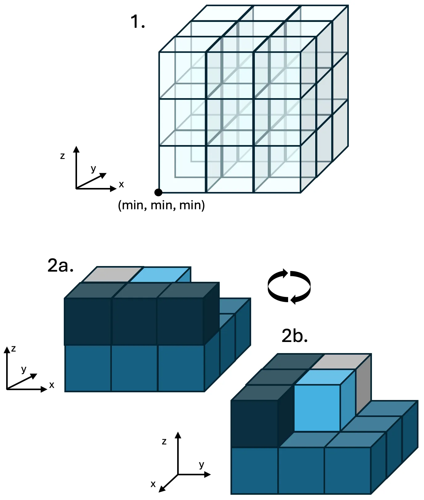For the LinkedCellContainer, this optimization requires some more thought. As shown in the picture above, for a specific Particle (light blue cell), we do not need to iterate over all of its neighboring cells, but only the unique cell pairs, as the other combinations will be computed and added later. To then only iterate over the unique Particle pairs within the relevant cells, the unique indices into the underlying storage are used.

In the end, the task of implementing the specialized iterators for each ParticleContainer, e.g. iterating over unique Particle pairs that lie within a specified radius, was a nontrivial task that robbed me of many hours of sleep.

Arithmetic Optimizations

std::pow Removal

In the profiling reports, I noticed a lot of time in our simulation was spent in std::pow, which could be improved drastically as we only used constant integer exponents. As a result, I inlined the computations with small exponents such as 2 or 3, and used ‘cached’ results for bigger exponents such as 12.

Square Roots

Within the force calculation, I removed the repeated square root which is an expensive operation. Adjusting the calculation to the squared values was straightforward and effective.

Vector<T, N> Improvements

I optimized this explicit data structure by adding compound operations, removing unnecessary temporarily created arrays or unnecessary loops, and added constexpr cases with less overhead for the most relevant instantiations of N=3 or N=2.

Compiler Toolchain (Lower Level) Optimizations

Loop Invariance

In the profiling report, I also noticed that an unusual lot of time was spent in end iterators, so I investigated a bit. I noticed, that the compiler could not verify that the call to proximityEnd() in the loop

for (auto it = proximityBegin(...); it != proximityEnd(); ++it) { ... } 

was loop-invariant, and thus executed this expensive call at each iteration. As a consequence, I manually pulled the call out of the loop.

Link-Time-Optimizations

Enabling LTO in release builds, which makes more complex compiler optimizations across translation units possible, decreased our execution time by 25%.

Experiment: Argon Crystallization

As the grand finale of the practical course, instead of some toy simulations, we needed to simulate an actual experiment with the tools we spent a semester implementing, and verify its physical properties—and fortunately I was responsible for that. Hence, I examined the cooling process of Argon and compared two very different cooling schedules: a gradual cooling process that should allow the atoms to arrange into a crystal, and a much faster supercooling process that should kinetically trap them.

FYI: The explanation of this experiment was essentially copied from the slides of our last presentation, and put into words.

Force Implementation

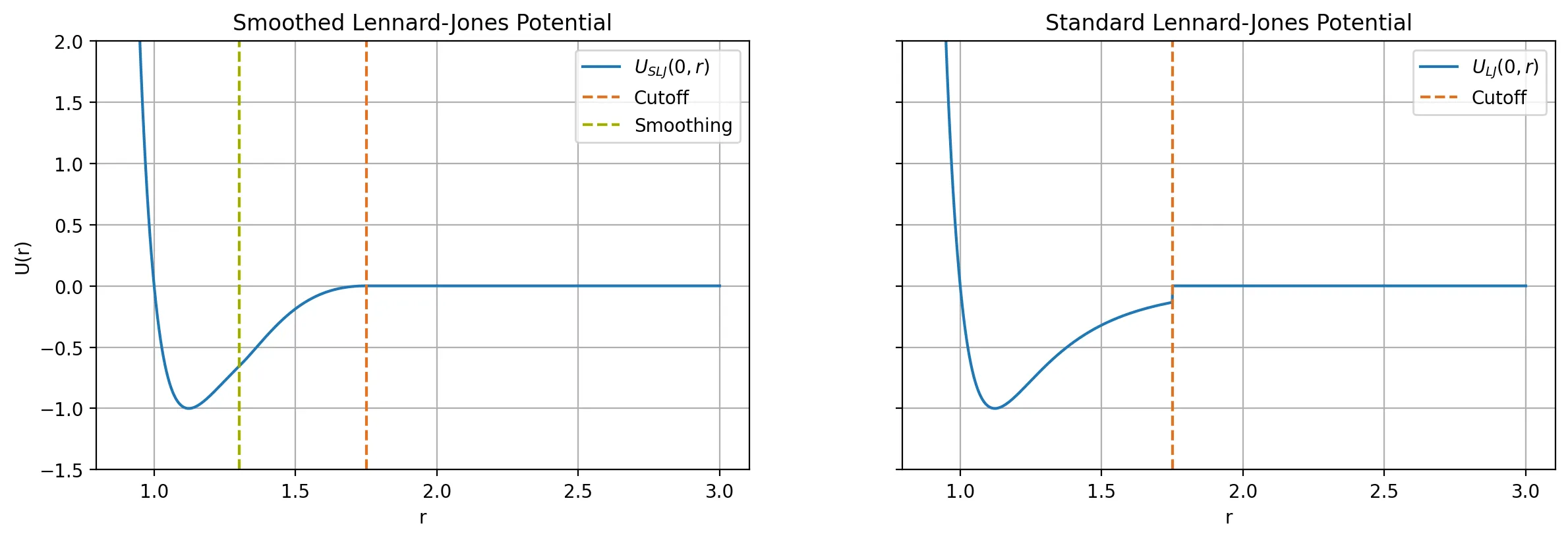
To simulate this process, I needed to implement one additional force that modelled the Smoothed Lennard-Jones Potential

using the standard Lennard-Jones potential and a smoothing function with a finite cutoff radius $r_c$ and a smoothing radius $r_l$

Below, the potentials are visualized:

Thermodynamic Statistics

To verify the behavior of Argon instead of relying only on the visual animation, I implemented the computation and collection of two thermodynamic statistics.

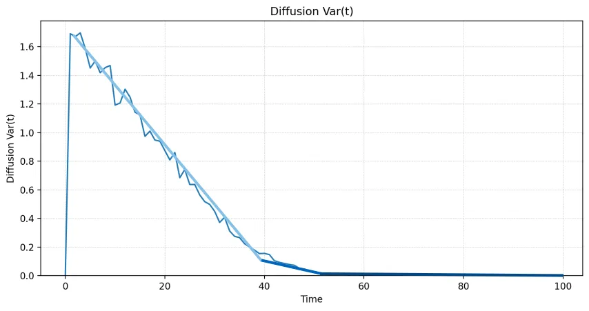
The diffusion

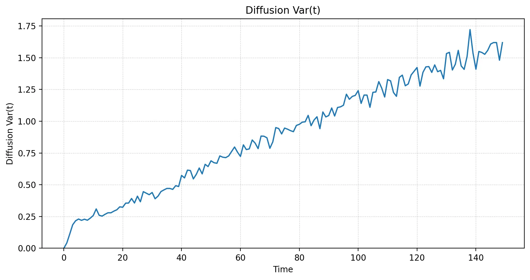
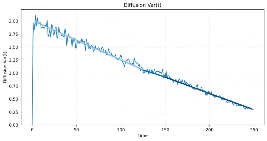
at a certain time is essentially a measure describing how far the particles are moving on average. A rapidly increasing value means that particles continue to move far from their reference positions; a flattening curve indicates that their mobility is being lost.

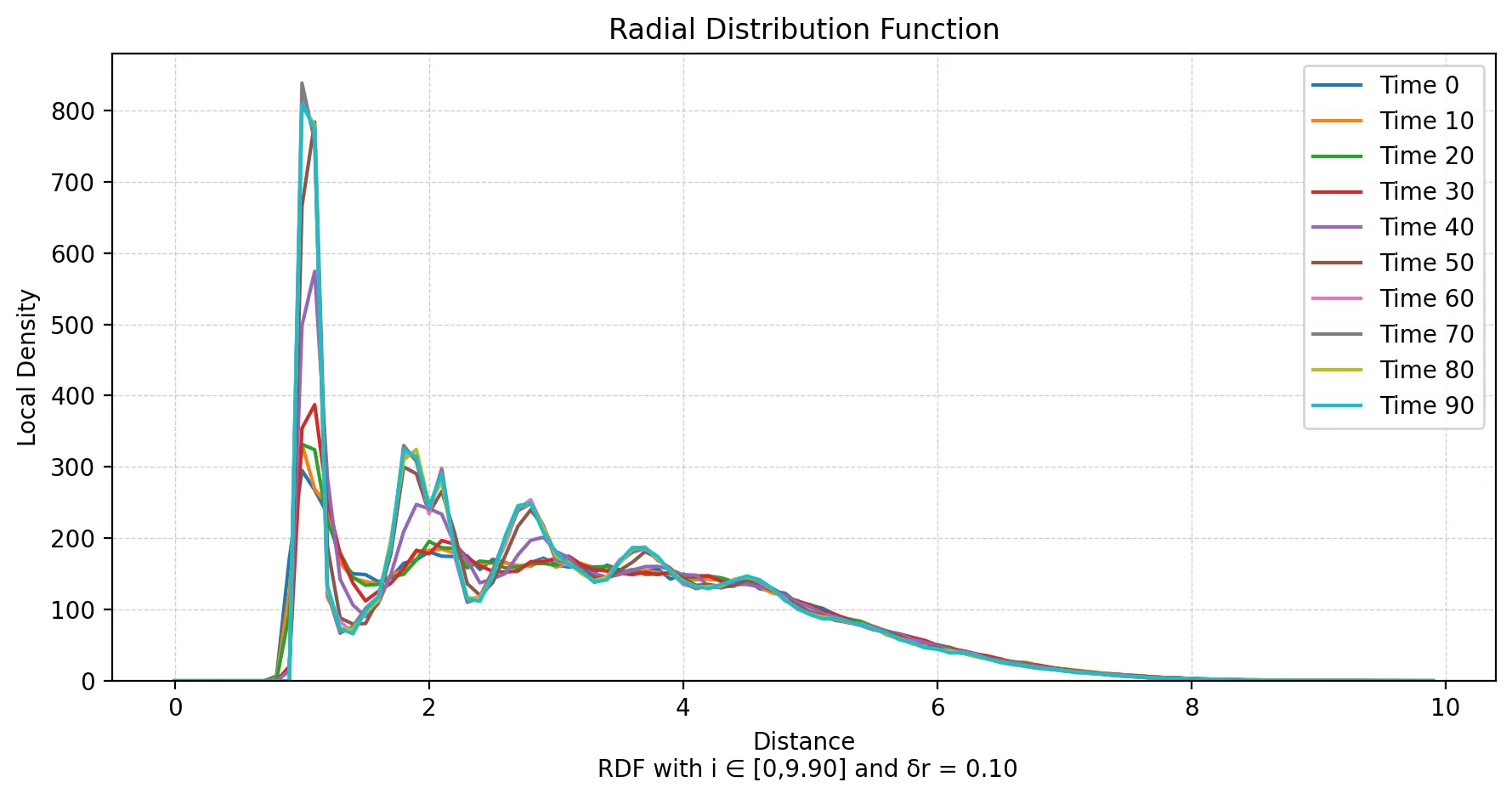
The radial distribution function (RDF)

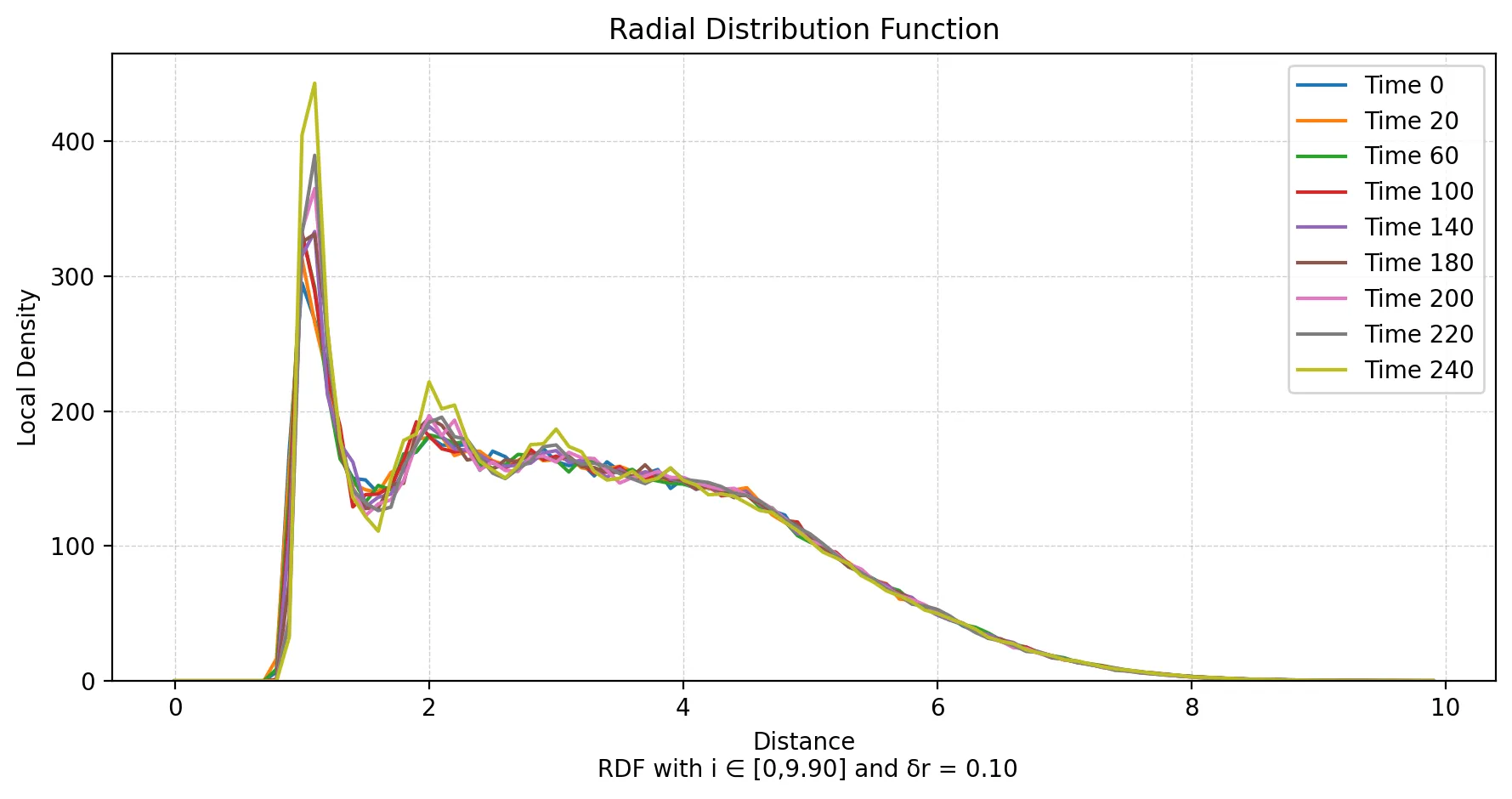
complements this with structural information. It maps each radial interval $[r_i,r_i+\delta r]$ to the local particle-pair density inside the corresponding spherical shell, with $N_{[r_i,r_i+\delta r]}$ being the number of particle pairs whose distance falls into that interval.

Simulation Setup

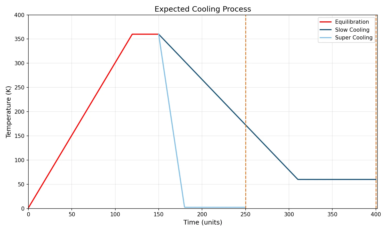
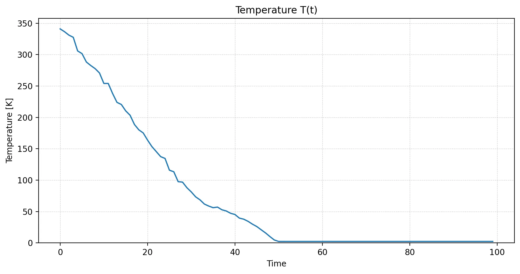
Both experiments began with the same equilibration phase at 360 K (86.85 °C). From that shared state, the slow-cooling run decreased the temperature to 60 K (−213.15 °C) over 250 simulation time units. The supercooling run instead plunged from 360 K to 2.4 K (−270.75 °C) in only 100 time units, as is abstractly visualized below:

Equilibration

Starting with a regular grid of particles and heating the system up over time, the diffusion statistic increased throughout this phase, meaning that the particles continued moving away from their stored reference positions as intended. The final checkpoint of this phase is used as a starting point for my cooling processes.

Slow Cooling Argon

Expectation

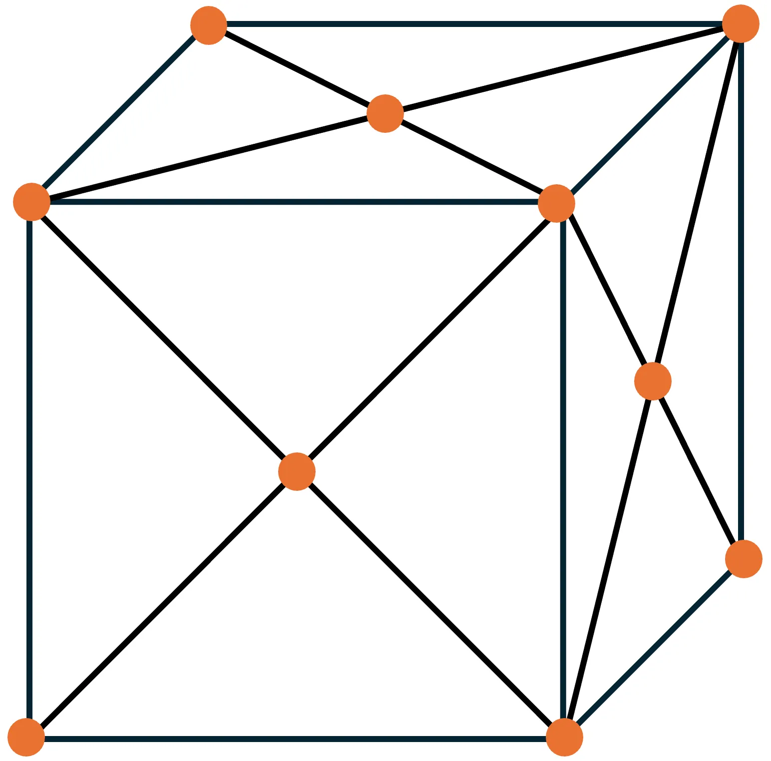
For the slow schedule, it was expected for the Argon to condense and eventually crystallize into a face-centered cubic (FCC) lattice. For reference, Argon’s condensation point is 87.3 K (−185.85 °C), while its crystallization point is 83.81 K (−189.34 °C) (source).

Expected FCC lattice structure	Extended view of the crystalline structure

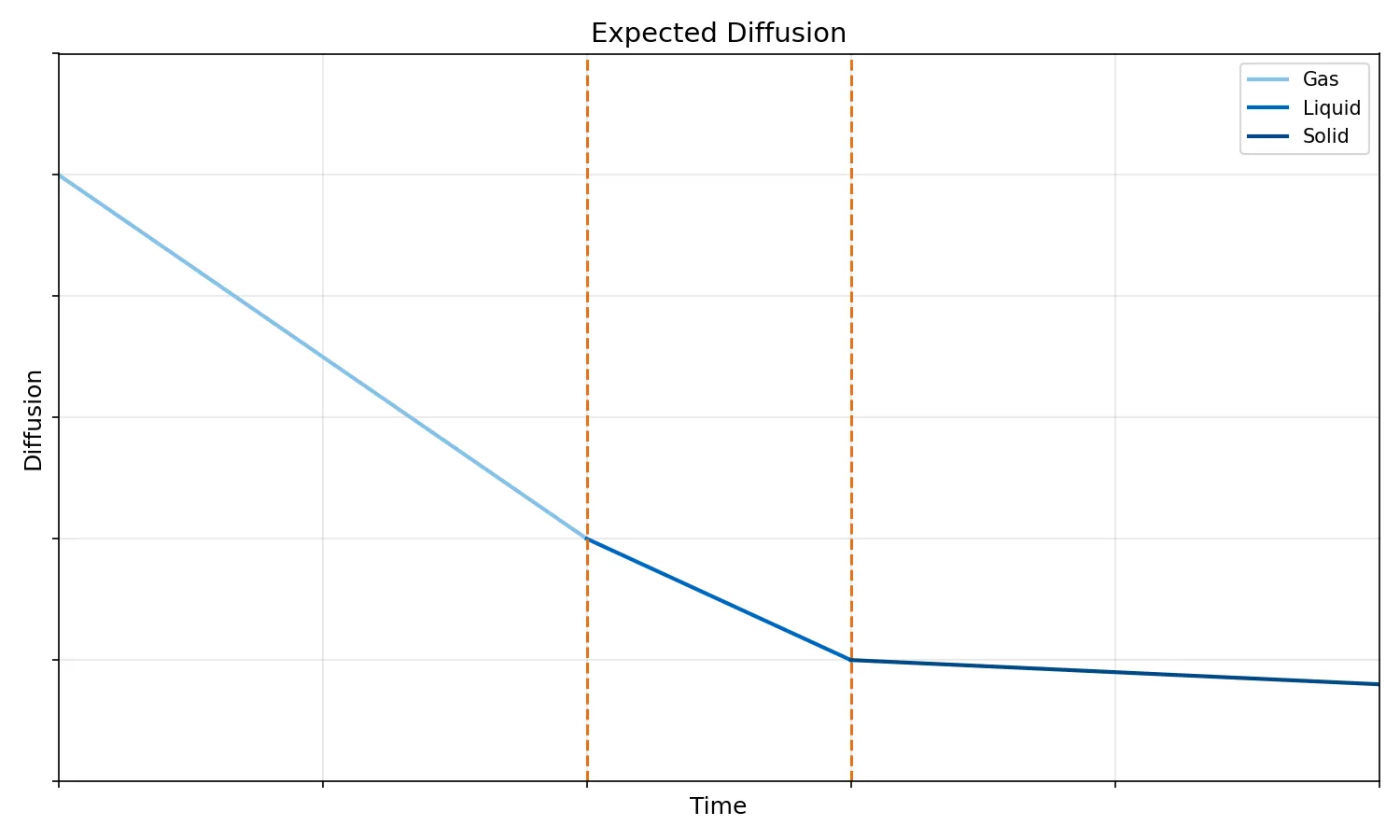
The diffusion curve should gradually flatten during cooling—lower temperature means less kinetic energy, which in turn means less particle movement. In an idealized picture, I expected piecewise, monotonically decreasing linear functions, as phase transition change the slope.

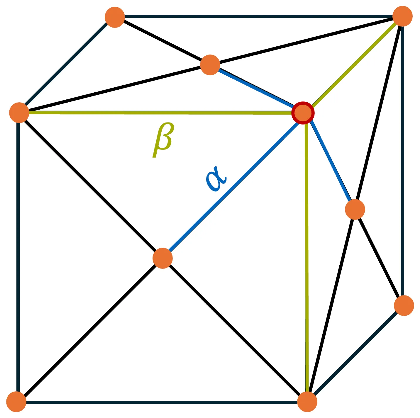
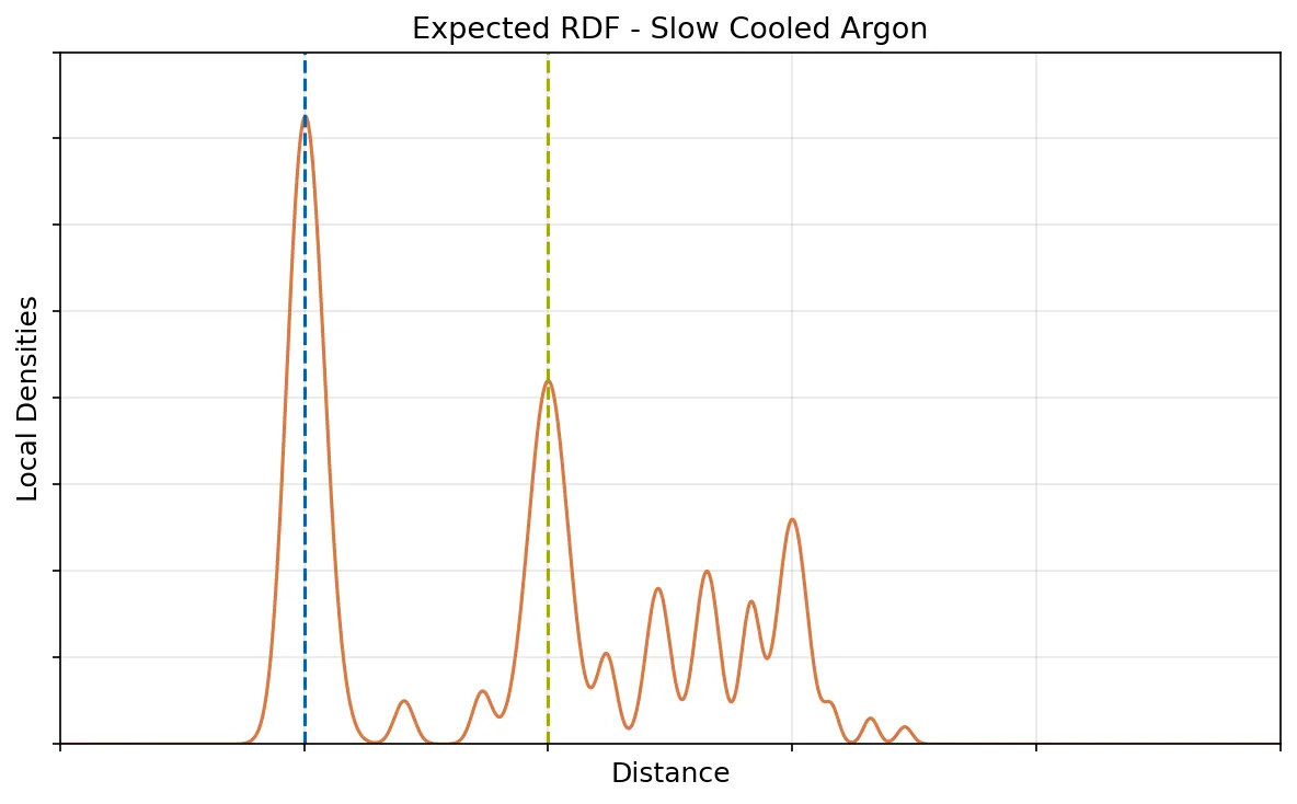
A crystal should also be visible in the RDF. Once atoms form a regular lattice, particular neighbor distances occur far more frequently than others. Distances such as $\alpha$ and $\beta$, and further lattice distances derived from them, should therefore appear as pronounced peaks.

Characteristic distances in crystalline Argon	Reference RDF for solid Argon

Result

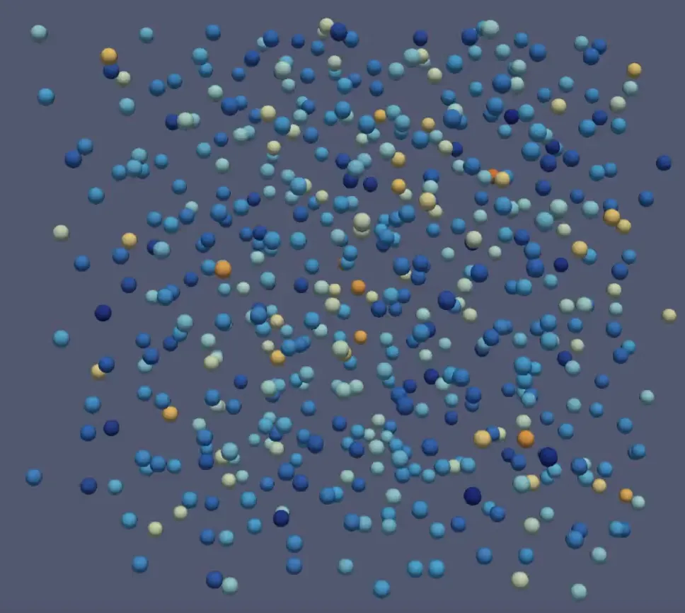
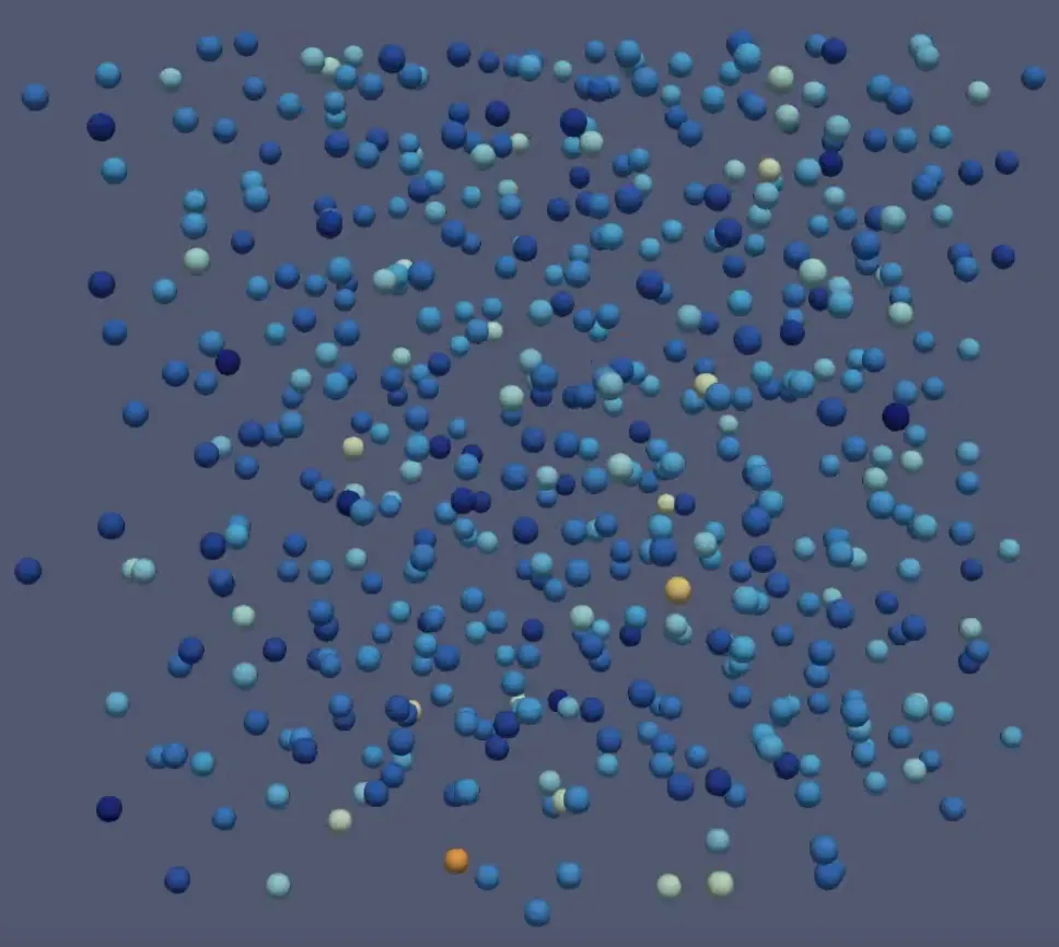
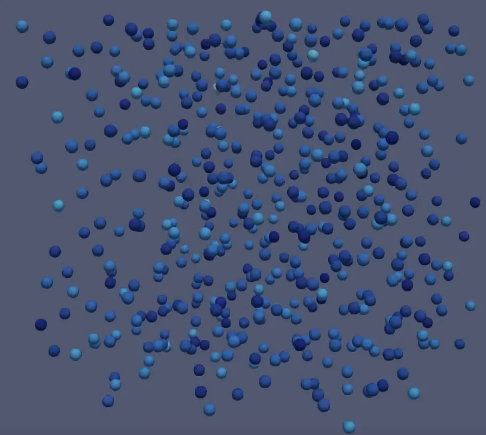
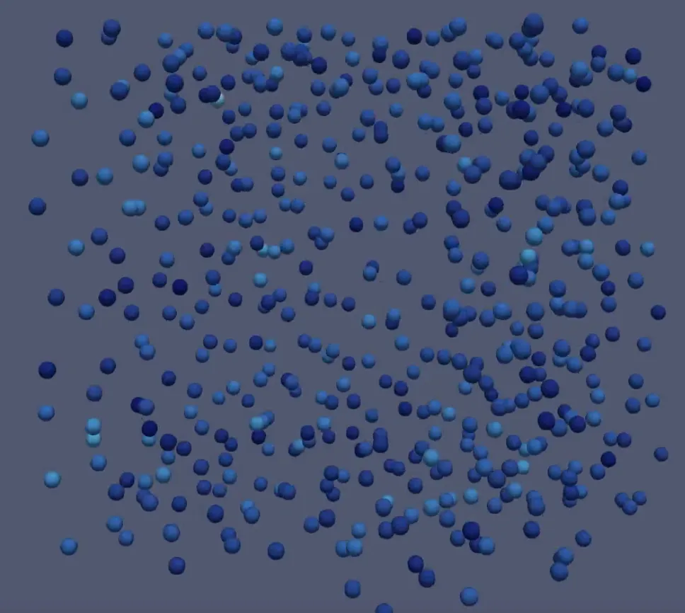
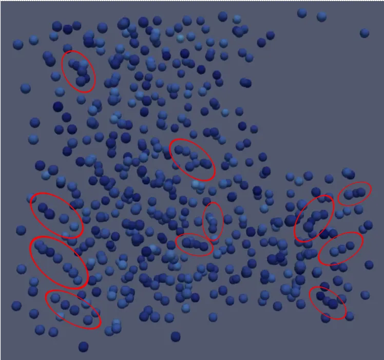
The animation of the original slow-cooling run, in which particle color represents velocity, unfortunately did not show crystallization clearly.

Initial equilibrated state	Video time 00:28	Video time 00:59	Final state

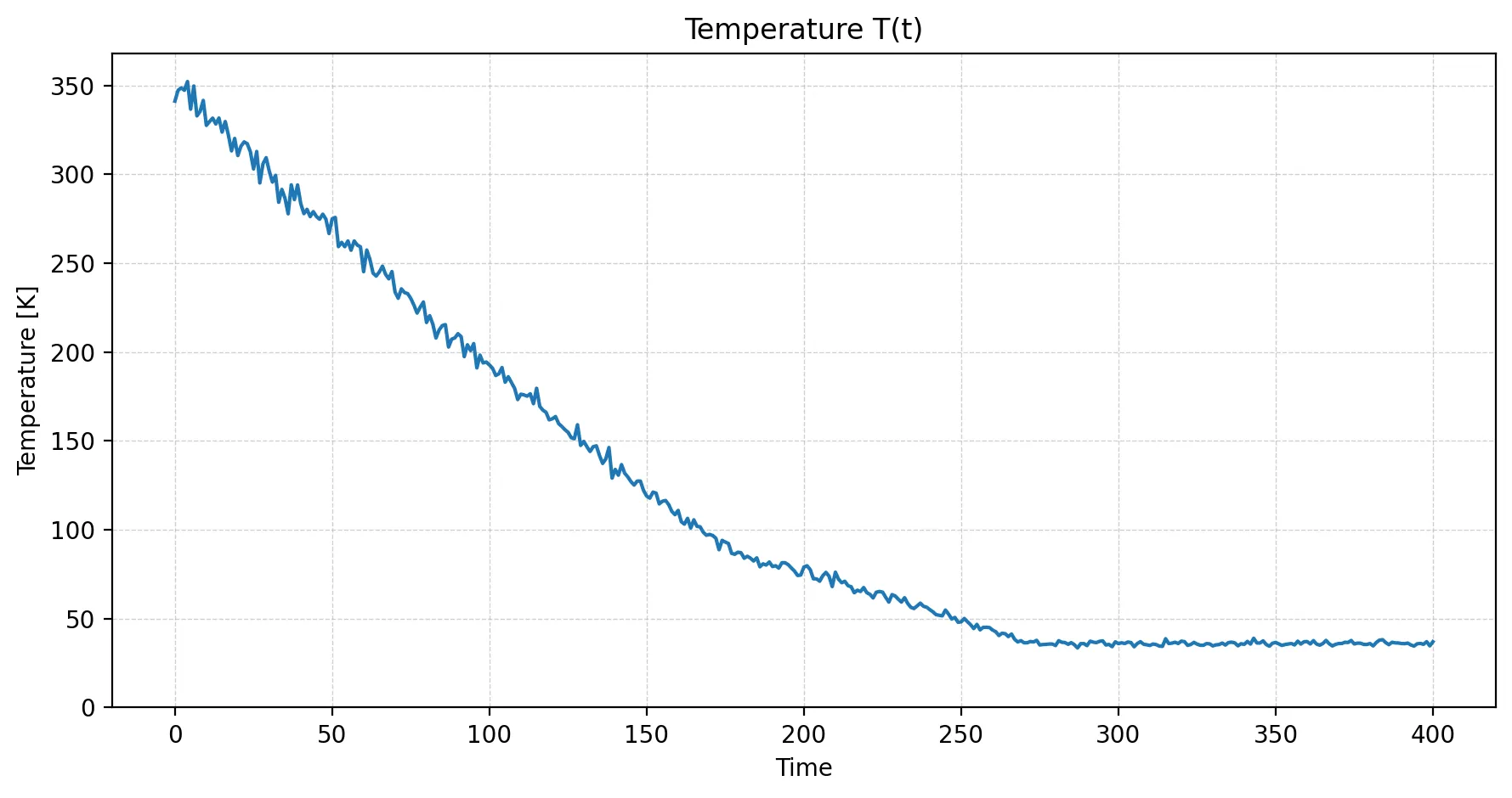
The temperature plot itself looked fine: it showed the requested shallow, linear decrease and reached the 60 K target. However, the system spent relatively little time below the crystallization point and did not end very far below it. Since we had no reference solution for this exact setup, I could not tell whether something was wrong or whether the Argon had simply been too warm for too much of the run.

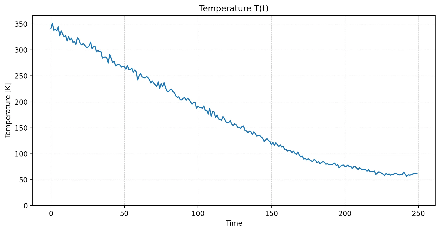
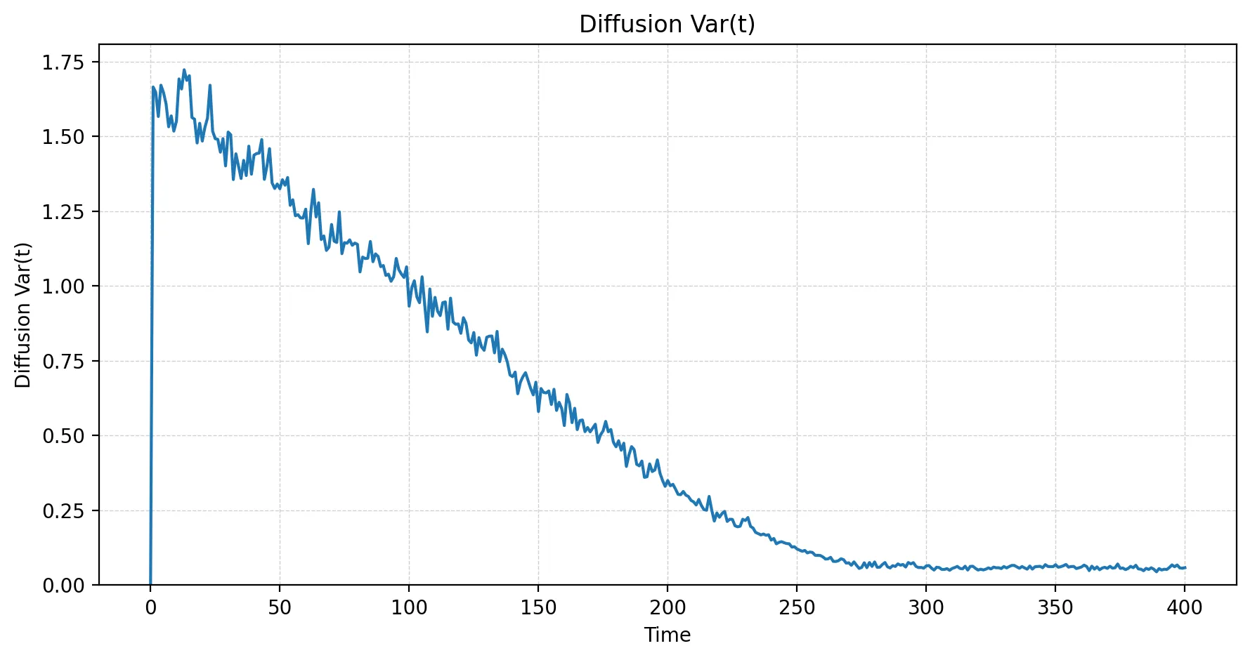
The diffusion data was as expected—mobility decreased during cooling, but the transitions between regimes were not super sharp.

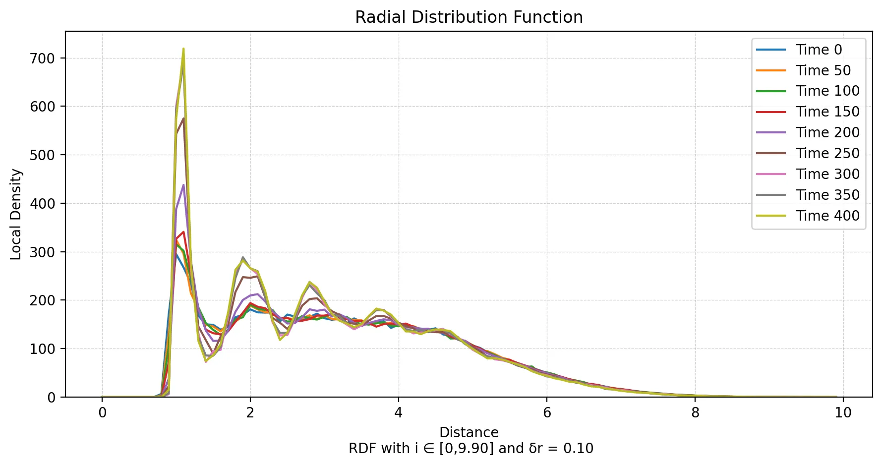
The RDF also showed the expected rise in local density and a significant first peak. Its later peaks, however, were not clearly concentrated at the characteristic lattice distances. The profile still looked more like that of a liquid, reinforcing the suspicion that crystallization had not truly started yet.

To test whether the system had simply been too warm, we performed an additional slow-cooling run with a lower target temperature of 36 K and observing the system far longer at this point. We kept the temperature decrement $\Delta T$ unchanged, so that the cooling rate remained the same. This put the target well below the crystallization point without going too close to absolute zero.

The animation with these adjusted parameters looked much closer to the expected crystalline behavior, as the final configuration image, RDF, and diffusion statistic suggest.

RDF after extended slow cooling	Diffusion after extended slow cooling

Super Cooling Argon

Expectation

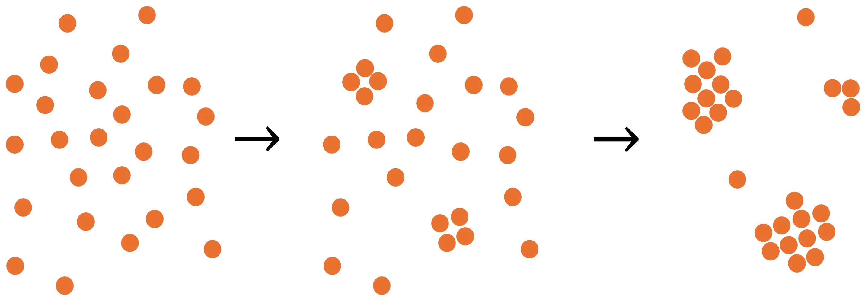
The fast schedule was intended to produce a very different outcome. Rather than giving the atoms enough time to arrange into an FCC lattice, the system was meant to “freeze” into a disorganized, liquid- or glass-like state, as is indicated below. Such a state is unstable in thermodynamic terms, but can persist because the particles are kinetically trapped.

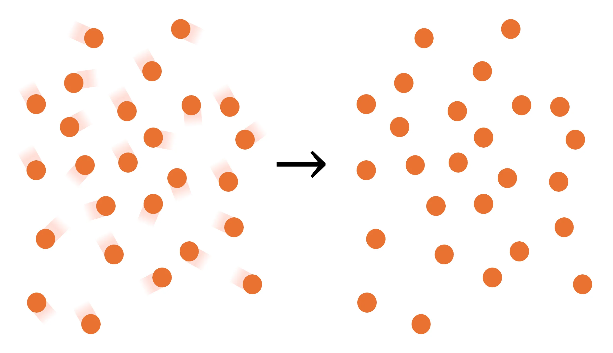
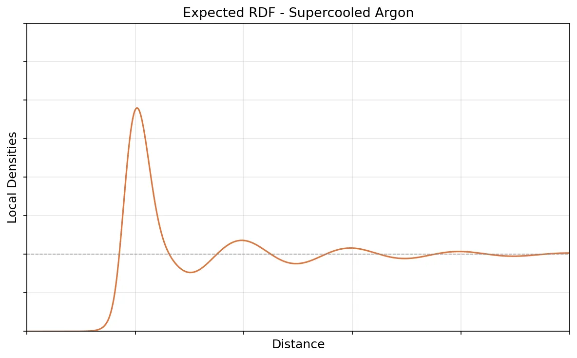
The much stronger temperature reduction should cause a correspondingly extreme loss of mobility, so that diffusion curve resembled that of the slow-cooling run, but with a substantially faster and more pronounced flattening. Structurally, the RDF should remain closer to a liquid RDF, so have fewer and less pronounced peaks overall.

Result

In the supercooling animation, the sudden “freeze” is clearly visible at about 00:15 in video time, corresponding to a simulated temperature of roughly 80 K. The system changes considerably between the 00:14 and 00:15 frames, but hardly changes after the 00:16 frame through the end of the run.

Initial equilibrated state	Video time 00:14	Video time 00:15	Video time 00:16

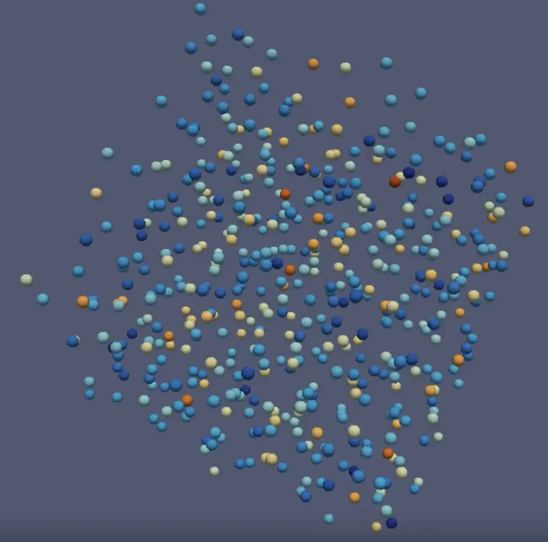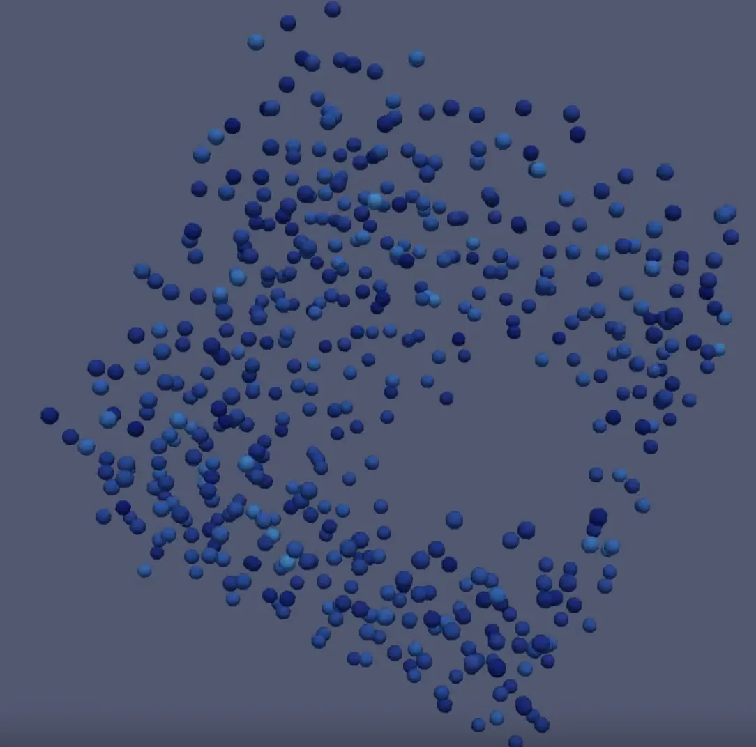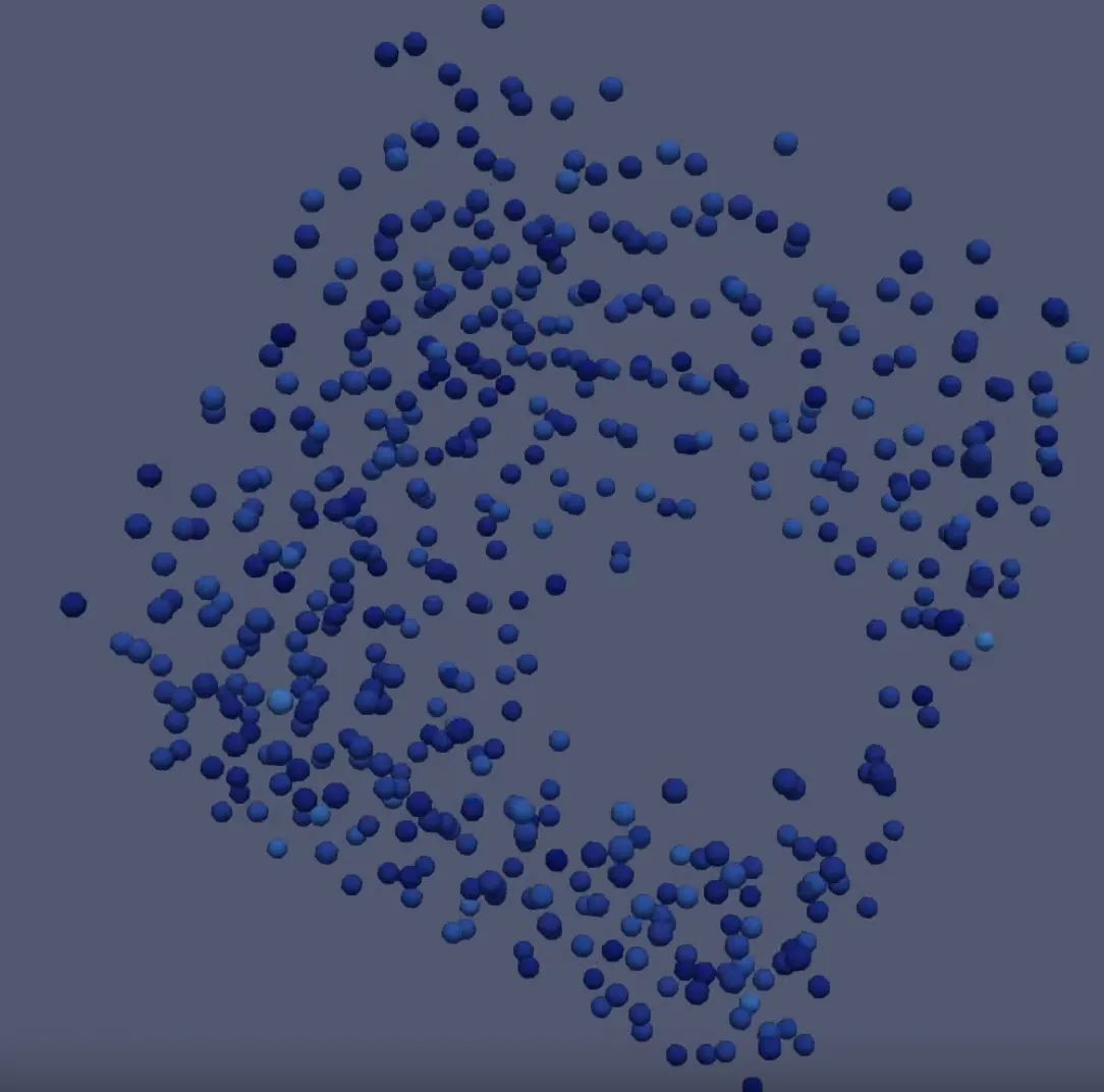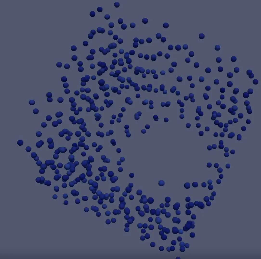As expected, the temperature fell linearly with a much steeper slope than in the slow-cooling experiment.

The diffusion statistic showed an extreme reduction in mobility during cooling. Near absolute zero there was almost no particle movement, and the transition was sharper than for slow cooling, matching the sudden visual freeze.

The RDF was less clear. The local densities increased and there was a significant first peak, as expected, but it also had more characteristic later peaks than we anticipated. Those could be signs of partial crystallization, but honestly, we did not have a definite explanation for them.

Acknowledgements

I really had a lot of fun working on this project, and my thanks go out to Henry and Georg—my amazing team mates. In my opinion, we really were on the same wave length and everyone carried the team in equal parts :)